Having a passion for image processing informs my work on machine vision projects and allows me to integrate my personal passions and professional expertise. Image processing intrinsically involves a lot of math and heavy computation. It is crucial to understand how and where you can optimize the code. This blog will introduce you to the basics of image processing.
Fair warning that I will introduce several mathematical concepts that you should understand to truly grasp image processing concepts, but they may not be necessary for algorithm implementation.
Terminology
- Pixel (aka picture element) - the smallest addressable element in a raster image.
- Kernel (aka convolution matrix, mask) - a matrix that allows you to manipulate images through convolution or cross-correlation.
- Convolution - an operation on two functions that produces an output function as described in the math section.
- Cross-correlation – similar to convolution but differs in the domain of operation as well as the preprocessing of input functions.
- Pixel weight – the level of contribution a given pixel has on the final output.
- Image noise – random variation of information within a given image.


Regular image (left) vs image containing excessive noise (right)
Convolution vs Cross-Correlation
When talking about image processing many people mistakenly refer to convolution in place of cross-correlation. Here is the mathematical representation of convolution, where you must invert the shifted multiplier.

Convolution
On the contrary, in cross-correlation, notice that we leave the shifted multiplier as is and instead take the complex conjugate of the main function, operation that would be ignored if working strictly in the real domain.

Cross-correlation

Cross-correlation in the real domain
It is quite important to note that convolution is commutative, where cross-correlation is not. That said, in reality, most if not all algorithms, technically, use cross-correlation instead of convolution (yes, including convolutional neural networks). You could potentially use either method, however, the output orientation will be an inverse of one another. This is because the preprocessing of each input function differs in the orientation.
The following is the convolution and cross-correlation visual demonstration. Kkeep in mind that the integral is going to be the same for two shifted multipliers that are opposite in the orientation, so this demonstration works for both operations depending on how you pre-process the shifted multiplier.
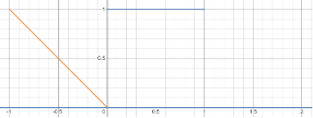
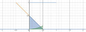
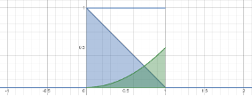
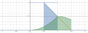
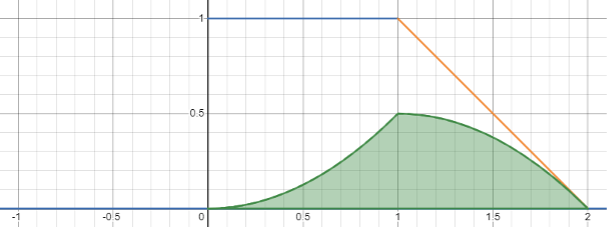
Blue unit function is the main function. Orange reverse identity function is the shifted multiplier. Blue area is the result of operation at a given moment. Green line is the output of cross-correlation (convolution).
Formats and Grayscale
There are multiple different formats that you can use to save your images.
- Raster images – images that have a predefined pixel proportion/density. You cannot resize these images without compromising the quality of the output. The common formats in this category are JPEG, GIF, PNG.
- Vector images – these images are constructed using proportional formulas, which makes them much more suitable for resizing. PDF, AI, SVG and EPS are such formats.
I will be focusing on raster images since they are direct representations of pixels and their locations. Additionally, to show image processing concepts, I will be utilizing grayscale images to avoid the complexity of dealing with multiple color channels.
There are different ways to convert a colored image into grayscale, however, my choice is ITU-R Recommendation BT.709.

R, G, and B – red, green, and blue channel intensities, respectively

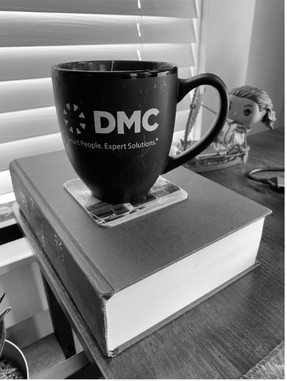
Color image vs grayscale image
Common Filters
Blur
There are different kinds of blurring techniques that are commonly used in image processing. To name a few: average, median, gaussian blurring. The main purpose of the blurring techniques is to reduce the noise of the image, or in other words to smooth the image out.
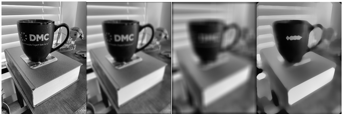 Left to right: original image, gaussian blur, average blur, median blur
Edge detection
Edge detection is another common algorithm that allows you to detect visible edges on a given image. This filter is commonly used in feature extractions of convolutional neural networks. You can detect edges in either x or y direction or choose both in parallel. You can also change the orientation of the edge detection from top to bottom and vice versa or from left to right and vice versa.
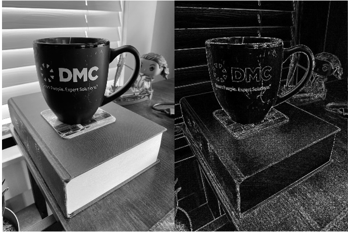
Original image vs edge detection outcome
Sandbox Setup
You can use the following code to build image processing algorithms. Python is my language of choice. It has extensive community support and a plethora of extremely helpful libraries that allow you to develop image processing concepts efficiently. However, you can utilize any language that you choose.
We will require the following libraries and classes to facilitate our algorithms:
import numpy as np
from PIL import Image
All the code will be defined within the parent ImageProcessor class that will outsource algorithms from helper classes. To run the code for testing we will set up a main function that will instantiate the ImageProcessor class that will give you access to desired functionality. For best practice, do instantiate the class in its own file.
from image_processor import ImageProcessor


if __name__ == "__main__":

    image_processor = ImageProcessor("images/dmc-mug.png")
Now, let’s see how you can set up the ImageProcessor class. The data to store in the ImageProcessor is the image data that will be required to produce desired results. Such data for now is the filename that will allow us to open the file, image in its original color code and the grayscale mode of the same image.
class ImageProcessor:

    def __init__(self, filename: str) -> None:

        # Image data.

        self.filename: str = filename

        self.image: np.ndarray = self.open_image(filename)

        self.gray_image: np.ndarray = self.to_grayscale(self.image)
To open, show, and save the images, you can use an external library called pillow. Do keep in mind that to save the images in the PNG format from a numpy array, you must cast the type, otherwise, you will get an empty image.
  def open_image(self, filename):

        with Image.open(filename) as raw_image:

            return np.array(raw_image.convert("RGB"))


    def save_image(self, filename, data):

        image = Image.fromarray(np.uint8(data))

        image.save(filename, "PNG")


    def show_image(self, image):

        img = Image.fromarray(image.astype(np.uint8))

        img.show()
Converting an image to grayscale can also be easily done like so:
 def to_grayscale(self, image):

        gray_image = np.zeros((image.shape[0], image.shape[1]))


        # ITU-R Recommendation BT.709: Y = 0.2126R + 0.7152G + 0.0722B - selected

        # ITU-R Recommendation BT.601: Y = 0.299R + 0.587G + 0.114B

        for r, row in enumerate(image):

            for p, px in enumerate(row):

                gray_image[r][p] = 0.2126 * px[0] + 0.7152 * px[1] + 0.0722 * px[2]


        return np.round(gray_image, decimals=0).astype(int)
Conclusion
Image processing might sound and look like a daunting task, but I’ve always found it very gratifying. The algorithms require lots of math and in-depth understanding of calculus which sounds intimidating, but it doesn’t have to be.
DMC would be happy to assist you with any software engineering endeavors utilizing years of experience in machine vision and Layer Imaging and Inspection Programming.
Learn about Custom Image Provider Implementation in PySide and contact us today for your next project.